Eikosograms: the picture of probability
- Online documentation is available here
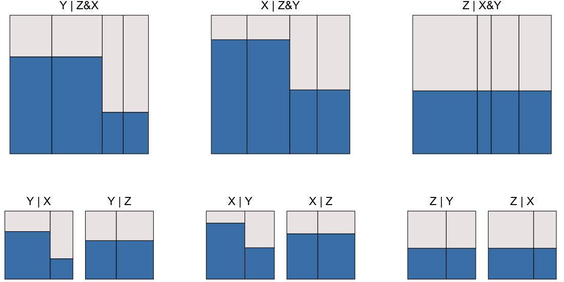
An eikosogram [eye-KOSS-oh-gram] (ancient Greek for probability picture) divides the unit square into rectangular regions whose areas, sides, and widths, represent various probabilities associated with the values of one or more categorical variates.
Rectangle areas are joint probabilities, widths are always marginal (though possibly joint margins, i.e. marginal joint distributions of two or more variates), and heights of rectangles are always conditional probabilities.
Eikosograms embed the rules of probability and are useful for introducing probability theory, including axioms, marginal, conditional, and joint probabilities, and their relationships (including Bayes theorem as a completely trivial consequence).
They are markedly superior to Venn diagrams for this purpose, especially in distinguishing probabilistic independence, mutually exclusive events, coincident events, and associations. They also are useful for identifying and understanding conditional independence structure.
As data analysis tools, eikosograms display categorical data in a manner similar to Mosaic plots, especially when only two variates are involved (the only case in which they are essentially identical, though eikosograms purposely disallow spacing between rectangles). Unlike Mosaic plots, eikosograms do not alternate axes as each new categorical variate (beyond two) is introduced.
Instead, only one categorical variate, designated the “response”, presents on the vertical axis and all others, designated the “conditioning” variates, appear on the horizontal. In this way, conditional probability appears only as height and marginal probabilities as widths. The eikosogram is therefore much better suited to a response model analysis (e.g. logistic model) than is a Mosaic plot.
Mosaic plots are better suited to log-linear style modelling as in discrete multivariate analysis.
Of course, eikosograms are also suited to discrete multivariate analysis with each variate in turn appearing as the response. This makes it better suited than Mosaic plots to discrete graphical models based on conditional independence graphs (i.e. “Bayesian Networks” or “BayesNets”).
Citation
If you use eikosograms in academic work, please cite the package:
citation("eikosograms")This will return the recommended citation for the software and the related unpublished manuscripts. The related unpublished manuscripts provide theoretical background, historical context, and pedagogical motivation for eikosograms and are available at: https://math.uwaterloo.ca/~rwoldfor/papers/eikosograms/.
