Introduction to eikosograms
R. W. Oldford
August 21, 2018
Source:vignettes/Introduction.Rmd
Introduction.RmdNote that eikosograms are grid objects and so may be
manipulated as any other (e.g. arranging several eikosograms in the same
display using grid.arrange() from the
gridExtra package).
library(eikosograms)
library(gridExtra)
A picture of probability
The word eikosogram is constructed by joining two ancient Greek words:
eikos: like truth, likely, probable, reasonable,
probability, likelihood
gramma: that which is drawn, picture, piece of
writing
As the name suggests, an eikosogram is a picture of probability. It visually partitions a unit square into rectangular regions whose areas give the numerical values of various probabilities. The construction is such that each rectangular region is identified with the value of one or more categorical variates.
For example, consider the probability that an application for admission to university is accepted. Different universities and programs of study can have different admission rates. For example, in 2017 there were about 15,200 applications to the Faculty of Mathematics at the University of Waterloo for only 1200 first year places, suggesting the probability that an application is accepted is about 0.08. Suppose this to be the case, then the eikosogram representing the application process is given by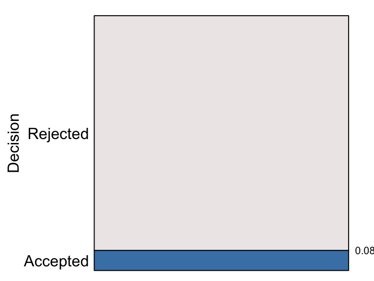
Application to Waterloo’s Faculty of Mathematics (2017)
Only two decisions are possible – an application is either accepted (and an offer of admission made) or it is rejected, as identified by the labels on the left side of eikosogram. On the right side of the eikosogram a single number appears, 0.08, marking the vertical height of the bottom (blue) rectangle.
An eikosogram always has unit area (whatever its aspect ratio) and
represents the totality of its probability with each side of the
eikosogram extending from 0 to 1. The bottom (blue) rectangle is
associated with the event that an application is accepted and its area
the probability of acceptance. This probability is determined by simply
calculating this area from the eikosogram as \[
\begin{array}{rcl}
Pr(Decision = Accepted) & = & width \times height \\
&& \\
& = & 1 \times 0.08 \\
&& \\
& = & 0.08
\end{array}
\] Since Decision is a binary variate, the top
(grey) rectangle is associated with the application being rejected. The
area of this rectangle is the probability \[
\begin{array}{rcl}
Pr(Decision = Rejected) & = & width \times height \\
&& \\
& = & 1 \times (1 - 0.08) \\
&& \\
& = & 0.92 .
\end{array}
\] These two areas give the probability distribution of the
binary random variate Decision whose value must be one of
\(\{Accepted, ~Rejected \}\). The
eikosogram gives a visual representation of this probability
distribution; the relative areas visually convey the magnitude of the
probabilities. Moreover, since the width of both rectangles is the same
(viz. 1) these probabilities are also given more simply (and visually
more accurately) by the heights of the two rectangles.
Grad admissions to Berkeley (1973)
A well known data set in R is UCBAdmissions
which records the number of applications and admissions to several large
graduate at the University of California (Berkeley) in 1973. This is a
table of counts cross classified by three different factors:
##  'table' num [1:2, 1:2, 1:6] 512 313 89 19 353 207 17 8 120 205 ...
##  - attr(*, "dimnames")=List of 3
##   ..$ Admit : chr [1:2] "Admitted" "Rejected"
##   ..$ Gender: chr [1:2] "Male" "Female"
##   ..$ Dept  : chr [1:6] "A" "B" "C" "D" ...
The eikos() function is used to produce the eikosogram
showing the probability of admission,
eikos("Admit", data = UCBAdmissions)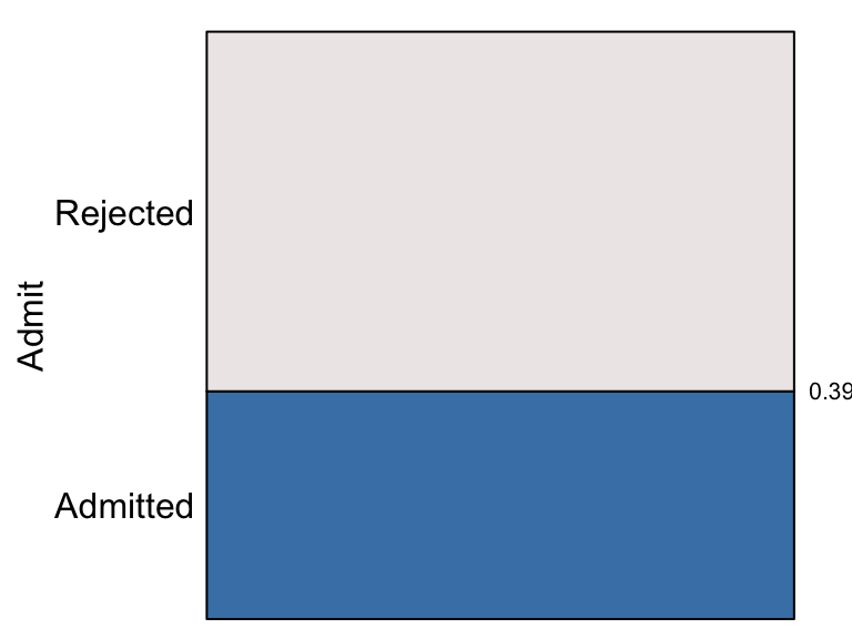
The proportion of applications admitted to these graduate programs at Berkeley in 1973 was 0.39. The probability of an application being admitted is represented by the area (or height) of the bottom (blue) rectangle and the probability of rejection by the area (or height) of the top (grey) rectangle which is 1 - 0.39 = 0.61.
The first argument to eikos() is the y or
“response” variate and determines the positions on the vertical axis.
There will be as many horizontal rectangles stacked up the vertical axis
as there are distinct values for y. For example, the
probability that any application is submitted to each of the six
graduate departments is
eikos("Dept", data = UCBAdmissions)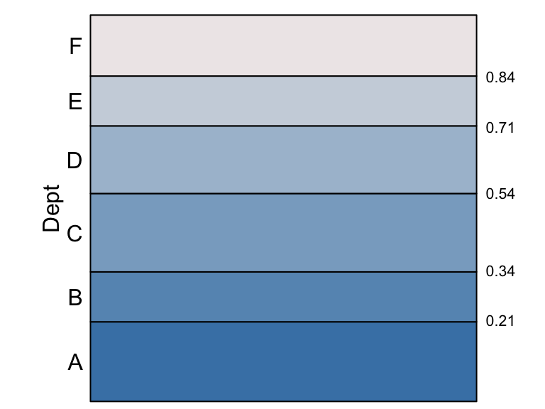
Again, areas correspond to probabilities and can be determined in
this case from each rectangle’s height (since widths are all 1). The
probability that a randomly selected application was submitted to
Department A is 0.21, to B is 0.13 (= 0.34 -
0.21), to C is 0.20 (= 0.54 - 0.34), to D is
0.17 (= 0.71 - 0.54), to E is 0.13 (= 0.84 - 0.71), and
finally to F is 0.16 (= 1 - 0.84).
Conditional and marginal probabilites
The eikosogram reinforces the basic probability rule that when the values of the variate are mutually exclusive and exhaust the set of possibilities, the probabilities must sum to one: \[Pr(Dept = A) + Pr(Dept = B) + \cdots + Pr(Dept = F) = 1 \] Note that this was because not all Berkeley departments are being considered here; these probabilities are therefore conditional on the fact that the department is one of the six largest.
In a very direct sense, the unit square of the eikosogram frames the probabilities expressed within it and these are always conditional on whatever background information determines the unit square.
For example, in addition to considering only the six largest departments, we could also restrict consideration by sex. The number of applications from each gender is
eikos("Gender", data = UCBAdmissions)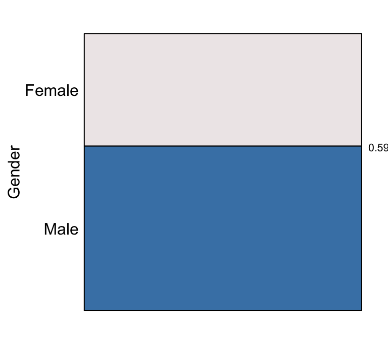
showing that there are unequal numbers of applications from each sex with \(Pr(Gender = Male) = 0.59\) and \(Pr(Gender = Female) = 0.41\).
The eikosogram conditional only on “Male” applicants is
eikos("Dept", data = UCBAdmissions[,"Male",],
      main = "Applications from males")
Probabilities can be determined as before but we can see immediately
from the eikosogram that departments A and B
are the most popular departments for male applicants, more so than for
all applications combined (in the previous eikosogram).
Conditioning on the “Female” applications
eikos("Dept", data = UCBAdmissions[,"Female",],
      main = "Applications from females")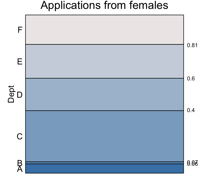
we see a rather different distribution of probabilities. Departments
A and B are much less popular with female
applicants than with male (e.g. only 1 in 100 applications from females
are to B compared to 1 in 5 for males). Instead departments
C and E are much more likely to receive an
application if it is from a female than if it is from a male.
Knowing the marginal probabilities that an application is from a female or a male, we might put these two eikosograms together in a single eikosogram.
eikos(y = "Dept", x = "Gender",  data = UCBAdmissions,
      xprobs_size = 8, yprobs_size = 8)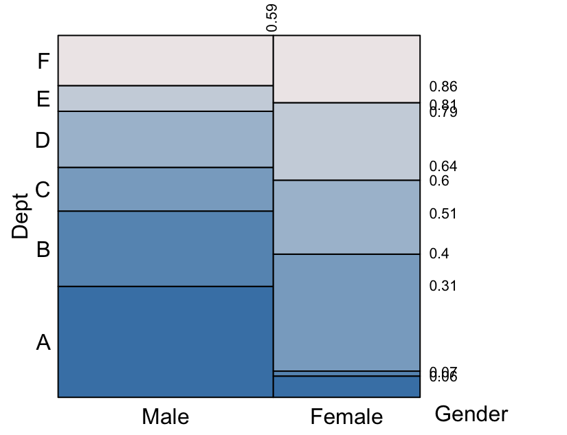
As can be seen the two conditional eikosograms are now fitted into the unit square, the width of each being the marginal probability of that conditioning variable “Gender”.
The conditioning variate(s) values appear across the bottom horizontal axis and the response along the left hand vertical axis. This arrangement makes reading the conditional probabilities follow visually left to right, top to bottom. For example, \(Pr(Dept = A ~\vert~Gender = Male) = 0.31)\) visually follows the display left to right and dropping down to the bottom edge for the value of the conditioning variate(s).
Numerical values along the top horizontal edge are the cumulative marginal probabilities associated with the values of the (bottom) conditioning variate. For example - the probability that an application is from a male applicant is \(0.59\) and - the probability that an application is from a female applicant is the difference \(1 - 0.59 = 0.41\).
Numerical values along the right vertical edge are the cumulative conditional probabilities for each department’s applications given gender.
For every horizontal line in the plot, the cumulative conditional probability to that height is given.
-
The height of each rectangle corresponds to the conditional probability of an application to that department given the corresponding gender. For example,
- \(Pr(Dept = E ~\vert~Gender = Male) = 0.86 - 0.79 = 0.07\)
- \(Pr(Dept = E ~\vert~Gender = Female) = 0.81 - 0.6 = 0.21\)
- \(Pr(Dept = A ~\vert~Gender = Male) = 0.31\)
- \(Pr(Dept \in \left\{B, D \right\} ~\vert~Gender = Male) = (0.51 - 0.31) + (0.79 - 0.64) = 0.35\)
-
The area of each rectangle corresponds to the joint probability of an application to that department from the corresponding gender. For example,
- \(Pr(Dept = E, Gender = Male) = 0.59 \times (0.86 - 0.79) = 0.0413\)
geometry and probability
In its construction, the eikosogram
- divides the unit square into
- vertical bars with widths equalling the probabilities for each value of the conditioning variate(s),
- and then divides each vertical bar horizontally into
- rectangles with heights equal to the conditional probabilities of each value of the response variate given the value(s) of the conditioning variate(s).
The area of every rectangle now equals the joint probability of the corresponding values of the conditioning and response variates.
The power of the eikosogram is that its geometry embeds the probabilities of discrete random variates:
the vertical axis shows the values of the response variate
the horizontal axis shows the values of the explanatory or conditioning variate(s)
each axis rangee exactly from 0 to 1
total probability is 1, the area of the whole eikosogram
widths of rectangles are marginal probabilities
heights of rectangles are conditional probabilities
-
areas of rectangles are joint probabilities
\[joint = area = height \times width = conditional \times marginal\]
the width of an entire vertical bar is the area of that bar (since its height is 1) and is also the sum of the areas of the rectangles it contains
the width of an entire vertical bar is the therefore the marginal probability for that value of the (horizontal) conditioning variate
By construction, probability comparisons are easily made visually with an eikosogram.
Marginal probabilities for the response
An eikosogram displays the joint probability of two (or more) categorical variates by area of rectangles. From this it is easy to determine the marginal probability of any value of the conditioning variate (width) but not the marginal probability of the response variate. This is because the heights record the conditional not the marginal probabilities of the response variate value given that of the conditioning variate.
The marginal for the response value is found by summing the areas of the rectangles having the same colour (i.e. those which correspond to the same response value).
This summing of areas is called marginalization and corresponds to a rule of probability. For example, \[Pr(Dept = A) = \sum_{gender \in \left\{Male, Female\right\}} Pr(Dept = A, Gender = gender)\] with \[Pr(Dept = dept, Gender = gender) = Pr(Dept = dept ~\vert~Gender = gender) \times Pr(Gender = gender) \] for all values of \(dept\) and \(gender\).
Marginalization can sometimes seems mysterious when first encountered. Fortunately, the eikosogram lends itself to another visual metaphor that simplifies the idea of marginalization. This is the water container metaphor.
the water container metaphor
Consider again the joint probability distribution of \(Dept\) and \(Gender\) given by the eikosogram
eikos(y = "Dept", x = "Gender", data = UCBAdmissions,
xlabs = FALSE, yaxs = FALSE, xaxs = FALSE)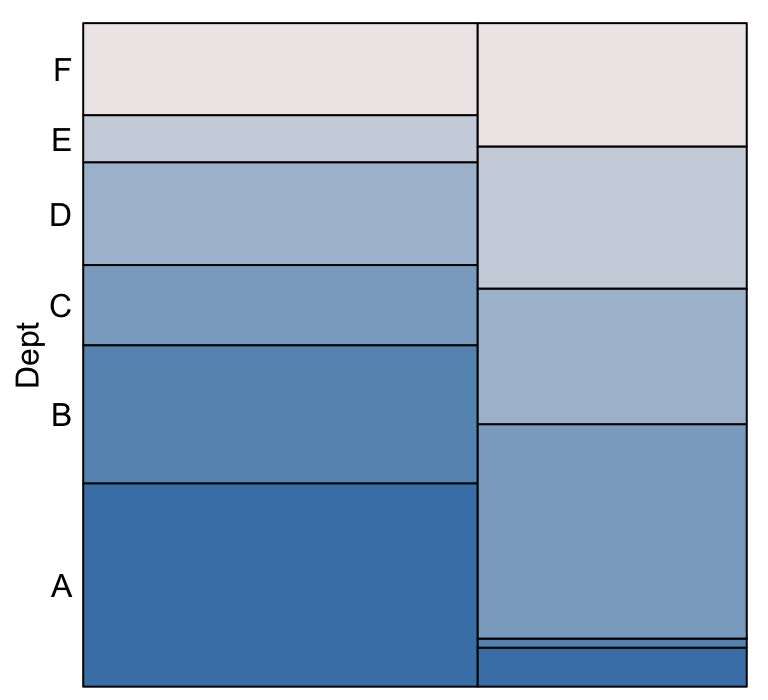 Only the department labels are shown and we now imagine that the picture
shows two containers beside one another, each containing liquids of
differing density so that the denser liquid, being heavier (and here
darker in colour), sinks to the bottom in each container. Each density
of liquid (colour of rectangle) corresponds to a department and each
container a gender (male on left, female on right).
Marginalization is simply removing the distinction between the two genders; or equivalently removing the barrier which separates the two containers. If these were liquids, then removing the barrier (or perforating the barrier) would cause the liquids to mix and then settle again according to density. The corresponding (now single combined) container would look like
eikos("Dept", data = UCBAdmissions,
      xlabs = FALSE, yaxs = FALSE, xaxs = FALSE)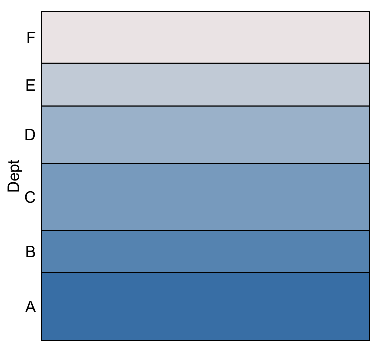
Just as the volume of each liquid must be conserved, so too must the area of each colour, and so the total probability for each department.
Marginalization can be thought of as perforating the barrier separating two volumes of liquid.
Bayes’s theorem
The eikosogram gives the joint probability of the response and conditioning variates. It highlights the marginal probabilities of the conditioning variate but not of the response variate, whose probabilities appear only as conditional. The appearance of the eikosogram, and hence the joint distribution, can be different depending on which variates are the response and which are conditioned upon.
For example, consider again the probability of admission to Berkeley graduate school, but this time condition on the sex of the applicant.
eikos(y = "Admit", x = "Gender", data = UCBAdmissions)
For all applications, this shows the joint distribution of the
variates Admit and Gender. As can be seen, the
probability of admission for male applicants is 0.45 and greater than
that for female applicants (0.3). The probability that an application is
from a male is 0.59 and from a female 0.41 = 1 - 0.59.
The joint probability that an application is from a male and that it results in an offer of admission is the area of the bottom left rectangle or
\[ \begin{array}{rcl} Pr(Gender = \mbox{"Male"} ~~\& ~~Admit = \mbox{"Admitted"}) &=& \mbox{area of bottom left rectangle} \\ &=& \mbox(height) \times \mbox{(width) of rectangle} \\ &=& Pr(Admit = \mbox{"Admitted"} ~\vert~Gender = \mbox{"Male"})\\ && ~~~~~~~~~~\times Pr(Gender = \mbox{"Male"} )\\ &=& 0.45 \times 0.59 \\ &=& 0.2655 \end{array} \] Similarly, the area of the bottom right rectangle is \[ \begin{array}{rcl} Pr(Gender = \mbox{"Female"} ~~\& ~~Admit = \mbox{"Admitted"}) &=& Pr(Admit = \mbox{"Admitted"} ~\vert~Gender = \mbox{"Female"}) \\ && ~~~~~~~~~~\times Pr(Gender = \mbox{"Female"} ) \\ & = & 0.3 \times 0.41 \\ &=& 0.123 \end{array} \] the area of the top left rectangle is \[ \begin{array}{rcl} Pr(Gender = \mbox{"Male"} ~~\& ~~Admit = \mbox{"Rejected"}) &=& Pr(Admit = \mbox{"Rejected"} ~\vert~Gender = \mbox{"Male"}) \\ && ~~~~~~~~~~\times Pr(Gender = \mbox{"Male"} ) \\ & = & (1 - 0.45) \times 0.59 \\ &=& 0.3245 \end{array} \] and finally the area of the top right rectangle is \[ \begin{array}{rcl} Pr(Gender = \mbox{"Female"} ~~\& ~~Admit = \mbox{"Rejected"}) &=& Pr(Admit = \mbox{"Rejected"} ~\vert~Gender = \mbox{"Female"}) \\ && ~~~~~~~~~~\times Pr(Gender = \mbox{"Female"} ) \\ & = & (1 - 0.3) \times (1 - 0.59) \\ &=& 0.287 \end{array} \] The sum of these four probabilities is of course 1.
Alternatively, the joint distribution of the variates
Admit and Gender could be expressed by
conditioning on the values or Admit rather than on those of
Gender:
eikos(y = "Gender", x = "Admit", data = UCBAdmissions)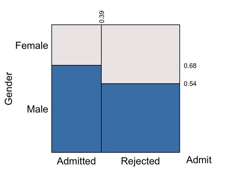
Now we see that the conditional probability that the the gender of the applicant was male given the application was admitted is 0.68. Given the application was rejected, the probability that the gender was male was only 0.54. The other two conditional probabilities, of the applicant being female, given the application was admitted or rejected is 0.32 amd 0.46 respectively.
These two eikosograms show the same joint
distribution and the four rectangles in each show the
same joint probabilities. That is the bottom left rectangle of
both eikosograms have the same variate values, namely the
Gender = “Male” and Admit = “Admitted”. They
must therefore have the same area. In the first eikosogram, this area
was \[
Pr(Admit = \mbox{"Admitted"} ~\vert~Gender =
\mbox{"Male"}) \times Pr(Gender = \mbox{"Male"} )
\] which is just $Pr(Admit = & Gender = ). The
same joint probability in the second eikosogram is the area of the
corresponding rectangle \[
Pr(Gender = \mbox{"Male"} ~\vert~Admit =
\mbox{"Admitted"}) \times Pr(Admit =
\mbox{"Admitted"}).
\] That these two rectangles have the same area is the famous
result due to the Thomas Bayes! Namely that \[
\begin{array}{rcl}
Pr(Admit = \mbox{"Admitted"} ~\vert~Gender =
\mbox{"Male"}) &\times& Pr(Gender =
\mbox{"Male"} )\\
= ~~
Pr(Gender = \mbox{"Male"} ~\vert~Admit =
\mbox{"Admitted"}) &\times& Pr(Admit =
\mbox{"Admitted"}).
\end{array}
\] Rectangles which identify the same joint probability
in both eikosograms must have the same area. This is Bayes’s theorem and
is perhaps most simply expressed generically as \[Pr(Y ~\vert~X) \times Pr(X) = Pr(X ~\&~ Y) =
Pr(X ~\vert~Y) \times Pr(Y).
\] Simply, areas of corresponding rectangles must match.
Independence
Two random variates \(X\) and \(Y\) are said to be distributed independently of one another if their corresponding eikosgram is flat.
For example, consider the following eikosogram
indep <- as.table(array(c(10, 40, 15, 60),
                        dim = c(2,2),
                        dimnames =
                        list(X =c("x_1", "x_2"),
                             Y = c("y_1", "y_2"))))
eikos("Y", "X", data = indep)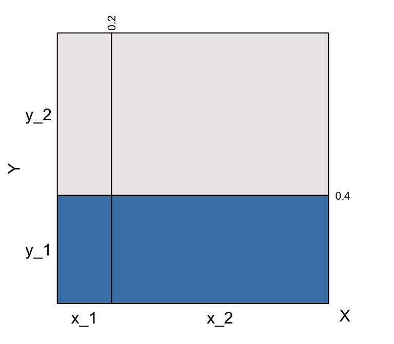
Independence of variates X and Y
Clearly, for \(i = 1, 2\) \[Pr(Y = y_i ~\vert~X = x_1) = Pr(Y = y_i ~\vert~X = x_2) = Pr(Y = y_i)\] This is what we mean by independence - whatever the value of \(X\) the probability that \(Y\) takes any particular value is the same. \(Y\)’s values are independent of those of \(X\).
By definition, this presents itself as all regions being flat across the values of the conditioning variate.
Of course, if we reverse the conditioning, flatness in the eikosogram must happen because of the independence. And this is what we see:
eikos("X", "Y", data = indep)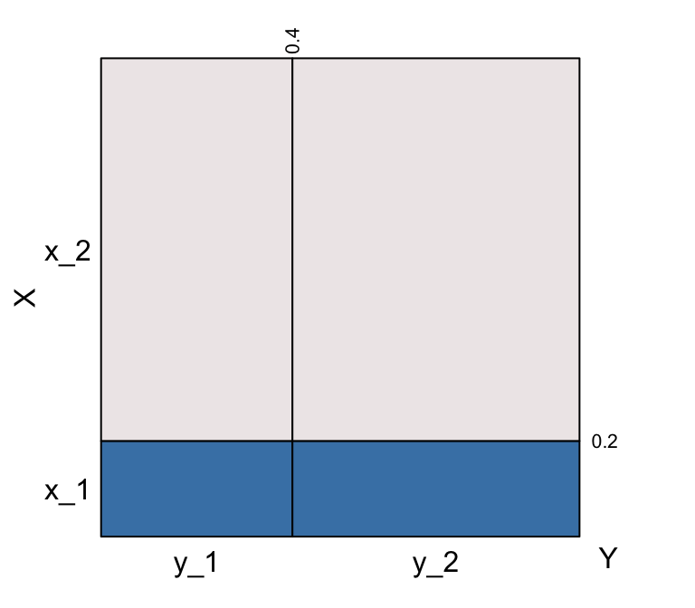
Independence of variates X and Y
Now, for \(i = 1, 2\) \[Pr(X = x_i ~\vert~Y = y_1) = Pr(X = x_i ~\vert~Y = y_2) = Pr(X = x_i).\]
It follows from either of these, and the definition that a joint probability is the area of the corresponding rectangle, that independence occurs if and only if for any \(i\), \(j\), \[Pr(X = x_i ~\&~ Y = y_j) = Pr(X = x_i) \times Pr(Y = y_j).\]
For a deeper exploration of independence relationships between categorical variates, see the vignette IndependenceExploration.
Events
Consider the possibility of two events, \(A\) and \(B\), each of which either occurs or does
not occur. Events simply modelled as binary variates taking values
Yes or No depending on whether the
corresponding event occurs or not.
As seen above, independence of two events occurs if and only all corresponding eikosograms are flat (see the vignette IndependenceExploration for more detail).
As with independence, a number of other fundamental reletionships between events uniquely present as eikosograms. This makes them both easily detected from the visualization and easily understood interpreted from the eikosogram. The concepts become clearly distinguished from one another (as opposed to Venn diagrams, see Cherry and Oldford (2003))
Coincident and complementary events
The visual hallmark of the eikosogram of a pair of events which are coincident, or of a pair which are complementary, is that the conditioning rectangles are all of one colour and are different from one another.
Coincident events If \(A\) and \(B\) are coincident events then the
eikosograms of their values (Yes for occurs;
No for does not occur) has the form:

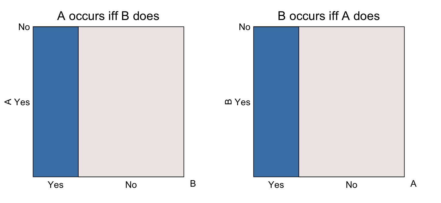
In the left most eikosogram, if event \(B\) occurs then \(A\) must occur (probability is 1); if the event \(B\) does not occur, then \(A\) cannot occur (probability is 0). The same information appears in the right hand eikosogram where \(A\) is now the conditioning event.
Complementary events If \(A\) and \(B\) are complementary events then the
eikosograms of their values (Yes for occurs;
No for does not occur) has the form:


In the left most eikosogram, if event \(B\) occurs then \(A\) cannot occur (probability is 0); if the event \(B\) does not occur, then \(A\) must occur (probability is 1). The same information appears in the right hand eikosogram where \(A\) is now the conditioning event.
Mutually exclusive events
Complementary events are a special case of mutually exclusive events. If \(A\) and \(B\) are complementary, then one of them must occur (in which case the other will not). \(A\) and \(B\) are mutually exclusive events, then if one occurs the other cannot however neither must occur. The eikosograms will look have the following form:

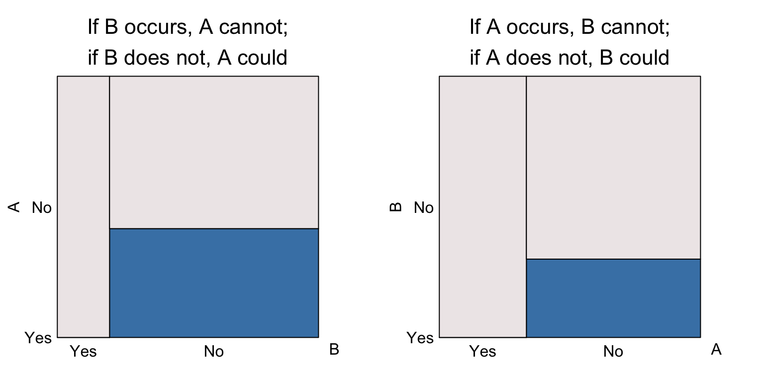
In the left most eikosogram, if event \(B\) occurs then \(A\) cannot occur (probability is 0); if the event \(B\) does not occur, then \(A\) may or may not occur (probability is greater than 0). The same information appears in the right hand eikosogram where \(A\) is now the conditioning event.
Mutually exclusive events only have some non-zero probability for the response event (vertical axis) occurring when the conditioning event does not. If that non-zero probability is also 1, then the events are complementary as well.
Positive and negative association
Between coincident and complementary events, we also remark on whether events tend to occur to gether or tend to not occur together. When events tend to occur together we say that they are positively associated; when they tend to not occur together we say that they are negatively associated.
Positive association If \(A\) and \(B\) are positively associated, their eikosograms will have the following form

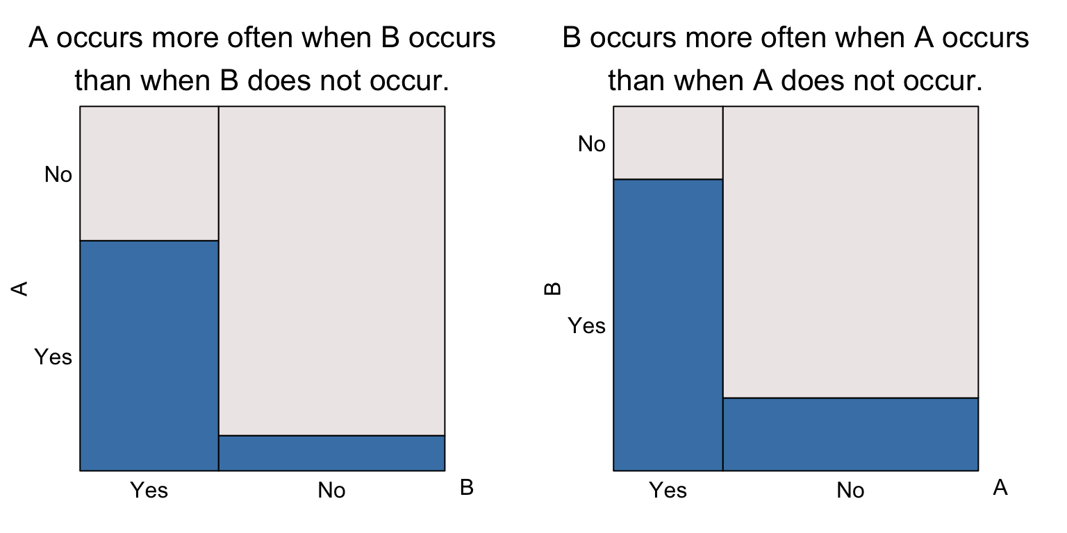
The visual hallmark is that the leftmost bar is higher than the rightmost. In the left eikosogram, this means that \[Pr(A \text{ occurs} ~\vert~B \text{ occurs}) > Pr(A \text{ occurs} ~\vert~B \text{ does not occur}).\] On the right eikosogram, we have the same for the other conditional probabilities, namely that \[Pr(B \text{ occurs} ~\vert~A \text{ occurs}) > Pr(B \text{ occurs} ~\vert~A \text{ does not occur}).\]
Clearly, coincident events are an especially strong case of positively associated events.
Negative association If \(A\) and \(B\) are negatively associated, their eikosograms will have the following form

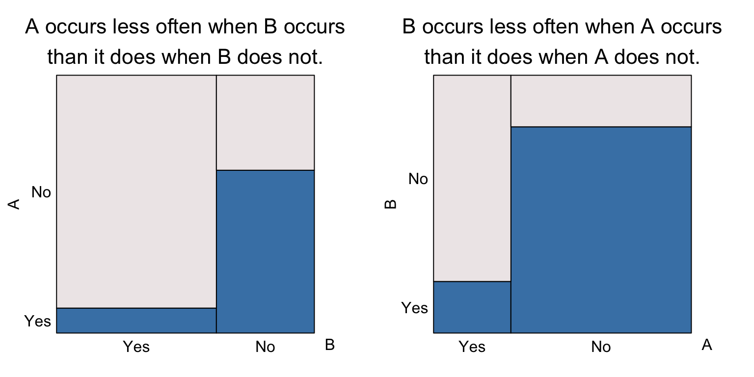
The visual hallmark is that the leftmost bar is lower than the rightmost. In the left eikosogram, this means that \[Pr(A \text{ occurs} ~\vert~B \text{ occurs}) < Pr(A \text{ occurs} ~\vert~B \text{ does not occur}).\] On the right eikosogram, we have the same for the other conditional probabilities, namely that \[Pr(B \text{ occurs} ~\vert~A \text{ occurs}) < Pr(B \text{ occurs} ~\vert~A \text{ does not occur}).\]
Clearly, complementary events are an especially strong case of negatively associated events.
An association spectrum
As the previous sections have shown, there is a range of associations that can be seen using eikosograms:


Here, the proportions have been arranged so that the total area of the bottom colour (i.e. blue) is the same across all five eikosograms. Similarly, the width of all columns are unchanged across the eikosograms. This has the effect that the marginal probabilities of the eventa are the same across all eikosograms.
The only differences between the eikosograms is in the association between the events. Applying the water container metaphor, it is only the distribution of the water between the two containers that has changed. Were the barrier between containers removed (or perforated so that the water can flow to an equilibrium), all resulting eikosograms would match that of the middle one (independence but without the vertical barrier). This reflects that the marginal probability of the event \(A\) occurring, or not, is identical in all five cases.
Conditional Independence
When there are more than two variates (or events) we can see
conditional independence of any pair given the values for the other
variate(s).
The key is to look for flat regions in the eikosogram where some
conditioning variate(s) values match.
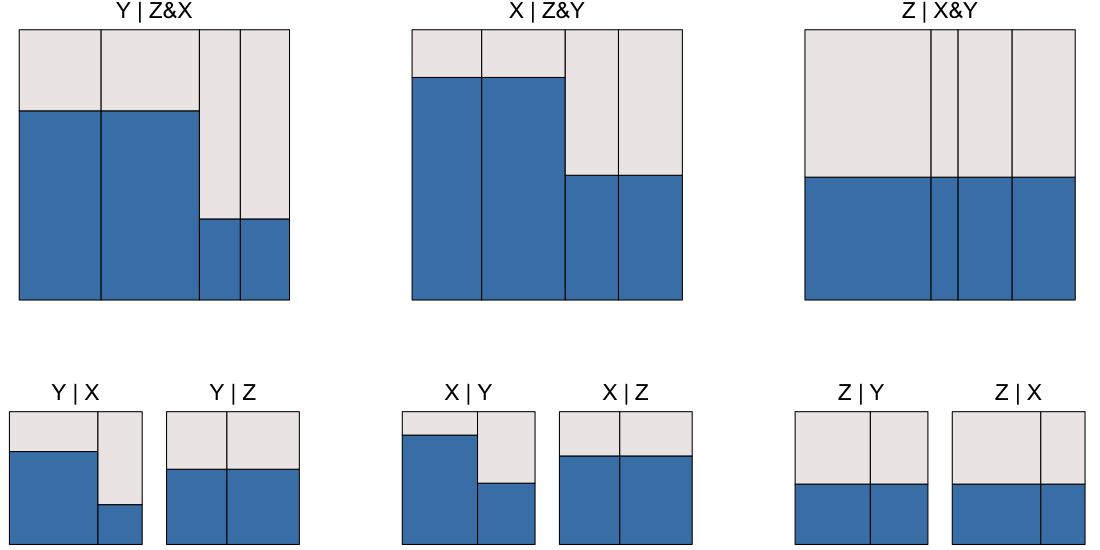
For example, consider the following eikosograms for the joint distribution of \(X\), \(Y\), and \(Z\), where each variate in turn appears on the vertical axiz as the response:


For the leftmost eikosogram, two flat regions appear. One occurs when \(Z = z1\) as \(X\) changes from \(x1\) to \(x2\). This flat region says that given \(Z = z1\), \(Y\) and \(X\) are independently distributed. The second flat region occurs when \(Z = z2\) and again for all values of \(X \in \{x1, x2 \}\). This implies that \(Y\) and \(X\) are also independently distributed when \(Z = z2\). When conditional independence between \(Y\) and \(X\) occurs for all values of the conditioning variate \(Z\), as it does here, we say that \(Y\) and \(X\) are conditionally independent given \(Z\).
This conditional independence makes it easy to see the conditional distribution of \(Y\) for each value of \(Z\). Applying the water container metaphor, this time removing the barriers between each value of \(X\) but preserving the barrier between the values of \(Z\), we see the joint distribution of \(Y\) and \(Z\) after marginalizing over \(X\). With these barriers erased, the leftmost eikosogram shows a negative association between \(Y\) and \(Z\) unconditionally on \(X\).
The middle eikosogram tells the same story, this time with \(X\) as the response variate. Again, the two flat regions demonstrate that \(X\) and \(Y\) are conditionally independent given \(Z\). Applying the water container metaphor as before, now reveals the joint distribution of \(X\) and \(Z\) after marginalizing over \(Y\). This reveals a posiitive association between \(X\) and \(Z\) unconditionally on \(Y\).
In the rightmost eikosogram, no flats appear and hence no conditional independencies exist. That is \(Z\) is neither conditionally independent of \(X\) given \(Y\) nor conditionally independent of \(Y\) given \(X\). Rather, in the rightmost eikosogram we can see that conditional on \(Y\) (for each of its values) \(Z\) and \(X\) are positively associated, and that conditional on \(X\) (for each of its values; note that the \(X\) values are not grouped) \(Z\) and \(Y\) are negarively associated.
For more investigation of conditional independence among three variates see the vignette IndependenceExploration.
Problems, puzzles, and paradoxes
Oldford (2003) contains a number of problems, puzzles, and paradoxes that are solved/explained via eikosograms. Many are classic problems, some are variations on these, and some are new. These include
- witness statement of a crime and the probability of guilt; the green cab blue cab problem from Tversky and Kahneman (1982)
- the gas station problem (a simplified version of the classic “secretary problem”)
- the “Cherry pie” paradox plus a new twist on it (this is a preference paradox involving ordering)
- a twice reversing Simpson’s paradox (artificially constructed)
- the two envelope problem
- the Monty Hall problem; and a new variation
- the prisoner’s dilemma (or three prisoner problem); and a new variation