Exploring Independence
R.W. Oldford
August 16, 2018
Source:vignettes/IndependenceExploration.Rmd
IndependenceExploration.Rmd
library(eikosograms)
library(gridExtra)
Independence
In this vignette, we explore independence and conditional independence between two or more categorical variates. It is recommended that the reader be familiar with the introduction to eikosograms vignette before continuing. Independence, including conditional independence is discussed there as well.
Of two variates
As discussed in the introduction to eikosograms vignette, the probabilistic independence of two categorical random variates clearly appears as a flat eikosogram. Two categorical random variates \(X\) and \(Y\) are distributed independently of one another if and only if their corresponding eikosgram is flat.
This is because independence is defined by the following relationship \[Pr(Y ~\vert~X) = Pr(Y) \] so that the conditional probabilities do not change as the value of the conditioning variate (\(X\)) change. In fact, the conditional probabilities are identical to the marginal probabilities (as if \(X\) were not there).
Equivalently, \(X\) and \(Y\) are independent if and only if \[Pr(X ~\vert~Y) = \Pr(X). \]
These mathematical equivalences arise as flat eikosograms are flat:
eikos("Y", "X", data = independenceExample)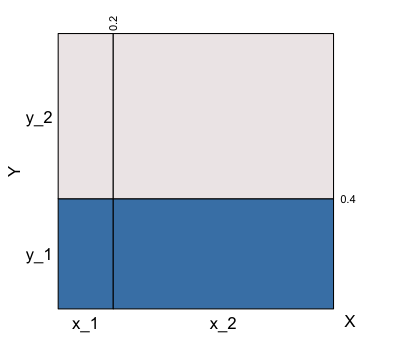
Independence of variates Y and X
eikos("X", "Y", data = independenceExample)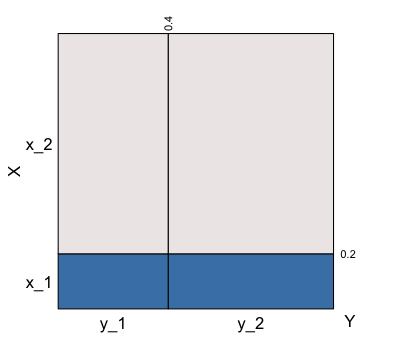
Independence of variates X and Y
Following Dawid (1979), we concisely denote the independence of \(X\) and \(Y\) by \(X \bot\hspace{-.5em}\bot Y\) or, being symmetric, equivalently \(Y \bot\hspace{-.5em}\bot X\). Similarly, when \(X\) and \(Y\) are known not to be independent we write \(X \bot\hspace{-.5em}\bot\hspace{-0.85em} \times Y\).
Note: In the example both \(X\) and \(Y\) were chosen to be binary random variates. This was done for two reasons.
- For simplicity of presentation: had there been more values of either \(X\) or \(Y\) there would have just been more columns in the eikosogram for the conditioning variate and more flat layers for the response variate.
- In some problems, we prefer to talk about events rather than random
variates. The same diagram can be used to discuss events: e.g. we could
define the event
Aas occurring wheneverX = x_1and not occurring whenX = x_2; similarly the eventBwould be defined as occurring or not wheneverYtakes valuesy_1ory_2respectively.
Conditionally
When we have three variates, say \(X\), \(Y\), and \(Z\), the pairwise independences \(Y \bot\hspace{-.5em}\bot X\), \(Y \bot\hspace{-.5em}\bot Z\), and \(Z \bot\hspace{-.5em}\bot X\) can be examined by looking at the corresponding eikosograms.
But we can also construct eikosograms that have more than one conditioning variate and so examine, for example, the conditional probabilities of \(Y\) given the pair of variates \(X\) and \(Y\). Some interesting features may result.
For example, consider the following eikosogram
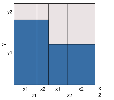
Conditional independence of variates Y and X given Z
The eikosogram has two flat sections, one when \(Z = z1\), the other when \(Z=z2\).
Looking only at the left hand flat first, we see from the eikosogram that \[Pr(Y ~\vert~X = x1 ~\&~Z = z1) = Pr(Y ~\vert~X = x2 ~\&~Z = z1)\] for all values of \(Y\). \(Y\) is therefore conditionally independent of \(X\) when \(Z = z1\), which we denote as \[ Y \bot\hspace{-.5em}\bot X ~\vert~(Z = z1). \] It follows mathematically that \[Pr(Y ~\vert~X ~\&~(Z = z1)) = Pr(Y ~\vert~Z = z1)\] for all values of of \(Y\) and \(X\).
Water container metaphor
This latter relation can also be observed directly from the eikosogram by applying the water container metaphor to the left hand flat.
To do so, think of the eikosogram as a series of columnar containers with a varying amounts of water each, as shown by the bottom blue rectangles (if \(Y\) had more values, think of the containers having liquids of various density to give the layers in each column). Were the boundary between two neighbouring containers to be perforated, then the liquid in the two containers would redistribute to find a new level across both containers.
If, for example, the boundary between the two neighbouring containers at left (between \(X = x1\) and \(X = x2\) when \(Z = z1\)) were to be removed, then the resulting level would unchanged. Removing this boundary removes the effect of changing \(X\) when \(Z = z1\); that is, we have marginalized over \(X\) with the resulting level becoming \(Pr(Y = y1 ~\vert~Z = z1)\). The unchanging level for this particular eikosogram implies the previous result, namely \(Pr(Y ~\vert~X ~\&~(Z = z1)) = Pr(Y ~\vert~Z = z1)\).
The same can be said about the right hand side of the eikosogram where \(Z = z2\). That is, it follows from the mathematics and/or eikosogram that we also have \[ Y \bot\hspace{-.5em}\bot X ~\vert~(Z = z2). \]
Since the conditional independence holds whatever value \(Z\) takes, we say more generally that \(Y\) and \(X\) are conditionally independent of one another given the value of \(Z\) and more succinctly write \[ Y \bot\hspace{-.5em}\bot X ~\vert~Z \] to assert that this holds no matter what the values of \(Y\), \(X\), or \(Z\).
Clearly a number of independence relationships are possiblie for any collection of three variates which suggests a broader notation for probabilistic independence might be of some help.
Independence when there are more than two variates
This section is a little technical and can be skipped. The next section focuses on only three variates and is illustrated via eikosograms.
When more than two variates are involved there are numerous ways in which the variates may exhibit some sort of independence, conditional and otherwise. Moreover, the conditional independence graphs do not capture all of these possibilities – see Oldford (2003) for demonstration and alternative graph representations.
However, the variants can be illustrated symbolically if we only slightly adjust the standard notation, switching from the standard “infix” use of \(\bot\hspace{-.5em}\bot\) to a “prefix” version.
A prefix notation for independence
\(X \bot\hspace{-.5em}\bot Y\) is the common notation to express the fact that random variates \(X\) and \(Y\) are probabilistically independent of one another.
A slight variant of this notation can be used to convey more than pairwise independence. The idea is to switch to using \(\bot\hspace{-.5em}\bot\) as a function of any number of variates. For a pair of variates \(\bot\hspace{-.5em}\bot(X, Y)\) means, as before, that \(X\) and \(Y\) are probabilistically independent of one another. The notation becomes useful when there it has more than two arguments (or variates); it then indicates that all variates are probabilistically independent in every way, a complete independence of one another. This idea is made more precise in this section.
Strictly speaking, the notation is not necessary to understand the rest of the vignette and readers may skip this subsection and return to it after observing eikosograms for the various possible cases of independence involving three variates. The notation principally permits these cases to be symbolically described more succinctly.
As an operator on two or more symmetrically treated variables, the function \(\bot\hspace{-.5em}\bot(X, Y, Z, \ldots)\) is understood as follows: \[\begin{eqnarray} \bot\hspace{-.5em}\bot(Y, X) & \mbox{ means } & Y \bot\hspace{-.5em}\bot X \nonumber \\ \bot\hspace{-.5em}\bot(Y, X)~\vert~Z & \mbox{ means } & Y \bot\hspace{-.5em}\bot X ~\vert~Z \nonumber \\ \bot\hspace{-.5em}\bot(Y, X, Z) & \mbox{ means } & \bot\hspace{-.5em}\bot(Y, X) ~\vert~Z, ~~ \bot\hspace{-.5em}\bot(Y, Z) ~\vert~X, ~~ \bot\hspace{-.5em}\bot(X, Z) ~\vert~Y,\nonumber\\ & & \bot\hspace{-.5em}\bot(Y, X), ~~ \bot\hspace{-.5em}\bot(Y, Z), ~ \mbox{ and } ~ \bot\hspace{-.5em}\bot(X, Z) \mbox{ all hold } \nonumber \\ & & \mbox{ or in the original (infix) notation, the following all hold: } ~~ \nonumber \\ & & Y \bot\hspace{-.5em}\bot X ~\vert~Z, ~~ Y \bot\hspace{-.5em}\bot Z ~\vert~X, ~~ X \bot\hspace{-.5em}\bot Z ~\vert~Y, ~~ Y \bot\hspace{-.5em}\bot X, ~~ Y \bot\hspace{-.5em}\bot Z, ~ \mbox{ and } ~ X \bot\hspace{-.5em}\bot Z \nonumber \end{eqnarray}\] When only the binary operation is called for, either the prefix or infix notation can be used depending on which seems clearer in the context.
As always, conditioning variables or events appear to the right of a vertical line (if more than one variable is conditioned on, as in Dawid (1979), they can appear listed separately within parentheses after the vertical bar).
The prefix notation \(\bot\hspace{-.5em}\bot(Y, \cdots , Z)\) is intended to indicate the complete probabilistic independence of its arguments which, as with pairwise independence, can occur for its arguments either unconditionally or conditionally given other random variables or events. So, \[\begin{eqnarray} \bot\hspace{-.5em}\bot(Y, X, Z) ~\vert~W & \mbox{ means } & \bot\hspace{-.5em}\bot(Y, X) ~\vert~(Z, W),~~ \bot\hspace{-.5em}\bot(Y, Z) ~\vert~(X, W),~~ \bot\hspace{-.5em}\bot(X, Z) ~\vert~(Y, W),~~ \nonumber \\ & & \bot\hspace{-.5em}\bot(Y, X) ~\vert~W, ~~ \bot\hspace{-.5em}\bot(Y, Z) ~\vert~W, ~ \mbox{ and } ~ \bot\hspace{-.5em}\bot(X, Z) ~\vert~W \nonumber \\ & & \mbox{ all hold } \nonumber \end{eqnarray}\] For four variables the recursive definition is \[\begin{eqnarray} \bot\hspace{-.5em}\bot(Y, X, Z, W) & ~~\mbox{ means that }~~ &\nonumber \\ & \bot\hspace{-.5em}\bot(Y, X, Z) ~\vert~W,& \bot\hspace{-.5em}\bot(Y, X, W) ~\vert~Z, ~~ \bot\hspace{-.5em}\bot(Y, Z, W) ~\vert~X, ~~ \bot\hspace{-.5em}\bot(X, Z, W) ~\vert~Y, ~~ \nonumber \\ & \bot\hspace{-.5em}\bot(Y, X, Z), & \bot\hspace{-.5em}\bot(Y, X, W), ~~ \bot\hspace{-.5em}\bot(Y, Z, W), ~~ \mbox{ and } ~~ \bot\hspace{-.5em}\bot(X, Z, W), ~~ \nonumber \\ & \mbox{ all hold. }& \nonumber \end{eqnarray}\] The extension of the notation to more than four variables is entirely analogous. \(\bot\hspace{-.5em}\bot\hspace{-0.85em} \times (Y, \cdots , Z)\) means that at least one of the independencies on the right hand side does not hold.
Given the number of independencies that are entailed, the phrase independence seems more evocative of the strength of the assertion than does the traditional independence. Oldford (2003) studies these relationships in some detail (including linking them to log-linear and graphical models).
The rest of the vignette explores eikosograms which show the various possible independencies that appear as part of the definition of \(\bot\hspace{-.5em}\bot(X,Y,Z)\).
Three variates
In this section we explore the possible independence relations between three variates.
Oldford (2003) provides some fake data constructed to illustrate the possible independence relationships between three categorical variates. For each example, there will be a table of joint probabilities from which eikosograms may be determined.
To simplify the presentation, each variate, \(X\), \(Y\), and \(Z\), will be binary, taking values “x1” or “x2”, “y1” or “y2”, and “z1” or “z2”, respectively. That way the number of combinations of variate values is reduced to \(8\), the number of cells in a complete \(2 \times 2 \times 2\) table of the joint probabilities.
A function to create the tables with data in the form given in the Appendix of Oldford (2003) is the following:
# This function will create all the joint probabilities
# and place them in the appropriate three-way table
create3WayBinaryTable <- function(widths, heights) {
    toprow_eikos <- widths * (1 - heights)
    bottomrow_eikos <- widths * heights
    probs <- array(c(bottomrow_eikos, toprow_eikos),
                  dim = c(2,2,2),
                  dimnames = list(Z = c("z1", "z2"),
                                  X = c("x1", "x2"),
                                  Y = c("y1", "y2")
                  ))
    as.table(probs)
}
Here the argument widths refers to the marginal joint
probabilities of the values of the conditioning variate pairs \((X, Z)\) in the order \((x1, z1)\), \((x1, z2)\), \((x2, z1)\), and \((x2, z2)\). The widths must sum to 1. The
argument heights gives the conditional probabilities of the
response variate \(Y\) taking value
\(y1\) for each of value of the
conditioning pairs \((X, Y)\) in the
same order as widths. There is no restriction on the
individual heights except that they be probabilities.
For example,
someTable <-   create3WayBinaryTable(widths =  c(10/35, 8/35, 5/35, 12/35),
                                     heights = c(7/10, 7/10, 7/10, 7/10))
produces the table of joint probabilities
| Z | X | Y | Freq |
|---|---|---|---|
| z1 | x1 | y1 | 0.2285714 |
| z2 | x1 | y1 | 0.1142857 |
| z1 | x2 | y1 | 0.1142857 |
| z2 | x2 | y1 | 0.1714286 |
| z1 | x1 | y2 | 0.0571429 |
| z2 | x1 | y2 | 0.1142857 |
| z1 | x2 | y2 | 0.0285714 |
| z2 | x2 | y2 | 0.1714286 |
from which, for example, the following eikosogram can be produced
(note that left to right in the eikosogram, the values of the
conditioning variates change from most to least frequently in the call
to eikos() according to the order in Which they appear in
its argument x).
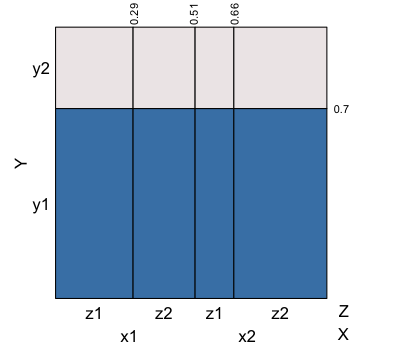
What is the independence structure?
This eikosogram suggests some sort of independence. Certainly, applying the water container metaphor makes it easy to see the “flat water” in the diagram implies that \(Y \bot\hspace{-.5em}\bot Z ~\vert~X\) and also that \(Y \bot\hspace{-.5em}\bot X ~\vert~Z\). That all of the levels are identical also allows us to see that any perforation of vertical barriers would have no effect on any of the heights and hence we can conclude that pairwise independencies \(\bot\hspace{-.5em}\bot(Y, X)\) and \(\bot\hspace{-.5em}\bot(Y, Z)\) also hold.
One might be tempted to jump to the conclusion that the flat structure across all values of \(X\) and \(Z\) implies that \(\bot\hspace{-.5em}\bot(X,Y,Z)\) also holds (i.e. that \(X\), \(Y\), and \(Z\) are completely independent). This would be a mistake. What this eikosogram fails to reveal immediately is the pairwise relationship between \(X\) and \(Z\) and what effect it might have, if any, on the remaining conditional relations \(X ~\vert~(Y, Z)\) and \(Z ~\vert~(X, Z)\).
It turns our that for this set of probabilities, the three variables \(X\), \(Y\), and \(Z\) are not completely independent.
The set of possibilities
For three variates, say \(X\), \(Y\), and \(Z\), a great many eikosograms are possibly of interest.
To begin with any one of the three variates can be chosen as the response variate (or vertical axis), with the combinations of the remaining two appearing as conditioning variates. The order of the conditioning variates (and possibly their values) could be rearranged to produce further variations in the display.
We also need to consider the eikosograms of every pair of variates unconditionally. That is, we need to consider the joint distribution of each pair without any consideration of the third variate (i.e. marginalizing over the third).
It turns out that there are only eight substantively different types of independence relationships between three categorical variates. When all three are binary variates, this is reduced to only seven possibilities. See Oldford (2003) for details and proofs. These seven possibilities will be illustrated in turn below.
Case 1: All three 3-way diagrams are flat
As was suggested earlier, it is not enough to consider only one of the variates as the response. While it may be possible to infer some independence structure from one three-way eikosogram, all three must be considered. If all three 3-way diagrams are flat, then \(\bot\hspace{-.5em}\bot(X, Y, Z)\) holds and we have complete independence.
An example where this occurs is very nearly the same as
someTable above and is given by the following table of
joint probabilities:
complete_indep <- create3WayBinaryTable(widths = c(10/33, 12/33, 5/33, 6/33),
                                        heights = c(7/10, 7/10, 7/10, 7/10))
The joint distribution can be shown in three different eikosograms depending on which variate is the response (for simplicity, none of the axis probabilities will be shown)
eikosY <- eikos(y="Y", x = c("Z", "X"),
                xaxs = FALSE, yaxs= FALSE,
                data = complete_indep, draw = FALSE)
eikosX <- eikos(y="X", x = c("Z", "Y"),
                xaxs = FALSE, yaxs= FALSE,
                data = complete_indep, draw = FALSE)
eikosZ <- eikos(y="Z", x = c("X", "Y"),
                xaxs = FALSE, yaxs= FALSE,
                data = complete_indep, draw = FALSE)
These can be displayed in a single figure using the function
grid.arrange() from the package gridExtra.
grid.arrange(eikosY, eikosX, eikosZ, nrow=1)
Complete independence
Note that each of the three eikosograms is completely flat. This is the hallmark of complete independence. In fact, it can be proved that \(\bot\hspace{-.5em}\bot(X,Y,Z)\) occurs if, and only if, all three of these 3-way eikosograms is flat.
The conditional independencies are obvious from the diagrams, as are the marginal pairwise independencies. To check the latter we could construct the corresponding histograms.
eikosYX <- eikos(y = "Y", x = "X",
                 data = complete_indep, main = "Y | X",
                 xaxs = FALSE, yaxs= FALSE, draw = FALSE)
eikosYZ <- eikos(y = "Y", x = "Z",
                 data = complete_indep, main = "Y | Z",
                 xaxs = FALSE, yaxs= FALSE, draw = FALSE)
eikosXZ <- eikos(y = "X", x = "Z",
                 data = complete_indep, main = "X | Z",
                 xaxs = FALSE, yaxs= FALSE, draw = FALSE)
grid.arrange(eikosYX, eikosYZ, eikosXZ, nrow = 1) 
Pairwise independence
For the other cases, it will be more convenient to produce all of these eikosograms at once. To that end, the following function will put simplified versions of all 3-way and all 2-way eikosograms together in one display.
layout3and2way <- function(table) {
    if(length(dimnames(table))!=3) stop("Must be a three-way table")
    varNames <- names(dimnames(table))
    zVar <- varNames[1]
    xVar <- varNames[2]
    yVar <- varNames[3]
    eikosY <- eikos(y = yVar, x = c(zVar, xVar),
                    data = table, main = paste0(yVar, " | ", zVar, "&", xVar),
                    xlabs = FALSE, ylabs = FALSE, xaxs = FALSE, yaxs= FALSE,
                    draw = FALSE)
    eikosX <- eikos(y = xVar, x = c(zVar, yVar),
                    data = table, main = paste0(xVar, " | ", zVar, "&", yVar),
                    xlabs = FALSE, ylabs = FALSE, xaxs = FALSE, yaxs= FALSE,
                    draw = FALSE)
    eikosZ <- eikos(y = zVar, x = c(xVar, yVar),
                    data = table, main = paste0(zVar, " | ", xVar, "&", yVar),
                    xlabs = FALSE, ylabs = FALSE, xaxs = FALSE, yaxs= FALSE,
                    draw = FALSE)
    eikosYX <- eikos(y = yVar, x = xVar,
                     data = table, main = paste(yVar, xVar, sep =" | "),
                     xlabs = FALSE, ylabs = FALSE, xaxs = FALSE, yaxs= FALSE,
                     draw = FALSE)
    eikosYZ <- eikos(y = yVar, x = zVar,
                     data = table, main = paste(yVar, zVar, sep =" | "),
                     xlabs = FALSE, ylabs = FALSE, xaxs = FALSE, yaxs= FALSE,
                     draw = FALSE)
    eikosXY <- eikos(y = xVar, x = yVar,
                     data = table, main = paste(xVar, yVar, sep =" | "),
                     xlabs = FALSE, ylabs = FALSE, xaxs = FALSE, yaxs= FALSE,
                     draw = FALSE)
    eikosXZ <- eikos(y = xVar, x = zVar,
                     data = table, main = paste(xVar, zVar, sep =" | "),
                     xlabs = FALSE, ylabs = FALSE, xaxs = FALSE, yaxs= FALSE, draw = FALSE)
    eikosZY <- eikos(y = zVar, x = yVar,
                     data = table, main = paste(zVar, yVar, sep =" | "),
                     xlabs = FALSE, ylabs = FALSE, xaxs = FALSE, yaxs= FALSE, draw = FALSE)
    eikosZX <- eikos(y = zVar, x = xVar,
                     data = table, main = paste(zVar, xVar, sep =" | "),
                     xlabs = FALSE, ylabs = FALSE, xaxs = FALSE, yaxs= FALSE,
                     draw = FALSE)
    layout <- rbind(c(1,1, NA, 2, 2, NA,  3, 3),
                    rep(NA, 8),
                    c(4, 5, NA, 6, 7, NA, 8, 9))
    grid.arrange(eikosY, eikosX, eikosZ,
                 eikosYX, eikosYZ,
                 eikosXY, eikosXZ,
                 eikosZY, eikosZX,
                 layout_matrix = layout,
                 widths = c(2,2,1,2,2,1,2,2),
                 heights = c(2, 0.5, 1.1)
    )
}
Calling this function on the complete_indep table, It is
clear that
layout3and2way(complete_indep)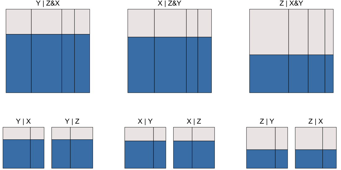
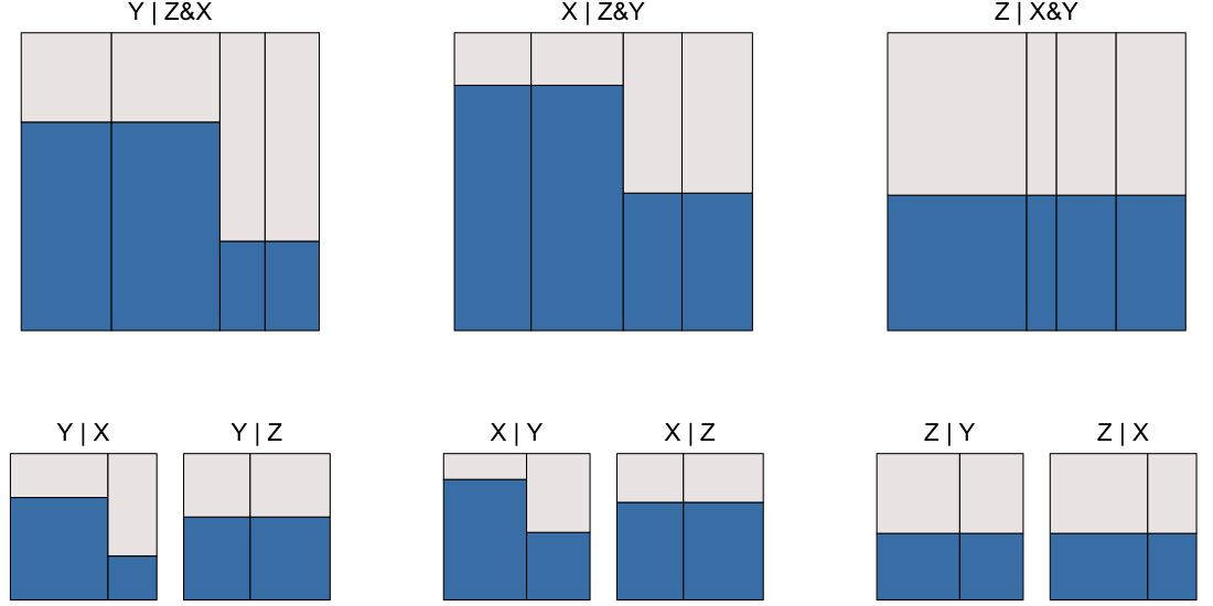
Complete independence
All eikosograms are flat, indicating the complete independence of all three variates from one another \(\bot\hspace{-.5em}\bot(X, Y, Z)\)
Case 2: one 4-flat, two 2 by 2-flats
As with the first case, it will be simplest to describe this by the shape of the 3-way eiksograms. In this case, one has the flar crossing all four conditions, the remaining two have flats crossing the values of one of the conditioning variates and not the others.
An example, and its simplified display is the following
table <- create3WayBinaryTable(widths = c(10/33, 12/33, 5/33, 6/33),
                               heights = c(7/10, 7/10, 3/10, 3/10))

layout3and2way(table)
One 4-flat; two 2 by 2 flats
Because not all eikosograms are flat, we can conclude that \(\bot\hspace{-.5em}\bot\hspace{-0.85em} \times (X, Y, Z)\); there are at least some dependencies amongst the three variates.
Recall that the value of the first conditioning variate mentioned changes fastest left to right across the vertical bars of any one eikosogram; the value of the second named conditioning variate changes more slowly.
Reading the top row of eikosograms from left to right, we see
- from the first top row eikosogram that
- \(Y \bot\hspace{-.5em}\bot Z ~\vert~X\), but that
- \(Y \bot\hspace{-.5em}\bot\hspace{-0.85em} \times X ~\vert~Z\);
- from the second eikosogram in the top row that
- \(X \bot\hspace{-.5em}\bot Z ~\vert~Y\), but that
- \(X \bot\hspace{-.5em}\bot\hspace{-0.85em} \times Y ~\vert~Z\); and
- from the third eikosogram in the top row that
- \(Z \bot\hspace{-.5em}\bot Y ~\vert~X\) and \(Z \bot\hspace{-.5em}\bot X ~\vert~Y\).
The second row reveals the joint dependence structure between two variates unconditionally, that is each eikosograms shows the joint distribution of the named pair of variates after marginalizing over the remaining third variate.
Reading the pairs of eikosograms in the second row from left to right we see
- from the first pair of eikosograms in the second row that
- \(Y \bot\hspace{-.5em}\bot\hspace{-0.85em} \times X\), but
- \(Y \bot\hspace{-.5em}\bot Z\);
- from the second pair of eikosograms in the second row that
- \(X \bot\hspace{-.5em}\bot\hspace{-0.85em} \times Y\), but
- \(X \bot\hspace{-.5em}\bot Z\);
- from the third pair of eikosograms in the second row that
- \(Z \bot\hspace{-.5em}\bot Y\), and
- \(Z \bot\hspace{-.5em}\bot X\).
In summary, the only independencies presented are
- \(Z \bot\hspace{-.5em}\bot X ~\vert~Y\),
- \(Z \bot\hspace{-.5em}\bot Y ~\vert~X\),
- \(Z \bot\hspace{-.5em}\bot X\), and
- \(Z \bot\hspace{-.5em}\bot Y\).
For the remaining cases, only the summary independencies will be provided.
Case 3: two 2 by 2-flats, one no-flat
This happens when there is only one conditional-independence.
table <- create3WayBinaryTable(widths = c(2/9, 1/9, 2/9, 4/9),
                               heights = c(2/3, 2/3, 1/6, 1/6))

layout3and2way(table)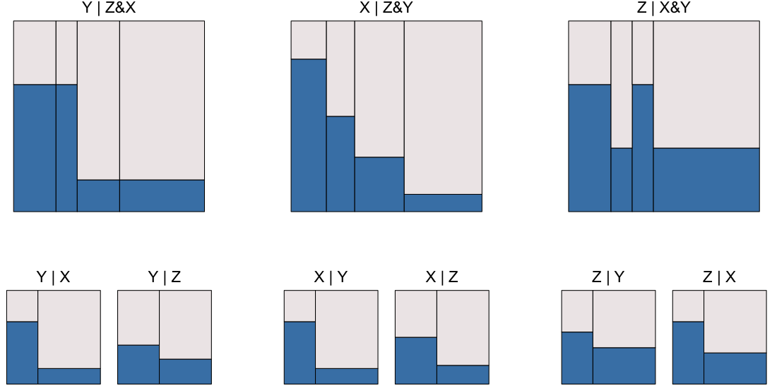
One no-flat; two 2 by 2 flats
Reading across the eikosograms, there is only a single independence relation of any kind, namely \(Y \bot\hspace{-.5em}\bot Z ~\vert~X\).
Case 4: three no-flats
Whenever no flat areas appear in the 3-way eikosograms, there are no conditional independencies.
Case 4.1: No flats; no marginal independence
table <- create3WayBinaryTable(widths = c(1/7, 1/7, 3/7, 2/7),
                               heights = c(1/3, 2/3, 1/4, 1/6))

layout3and2way(table)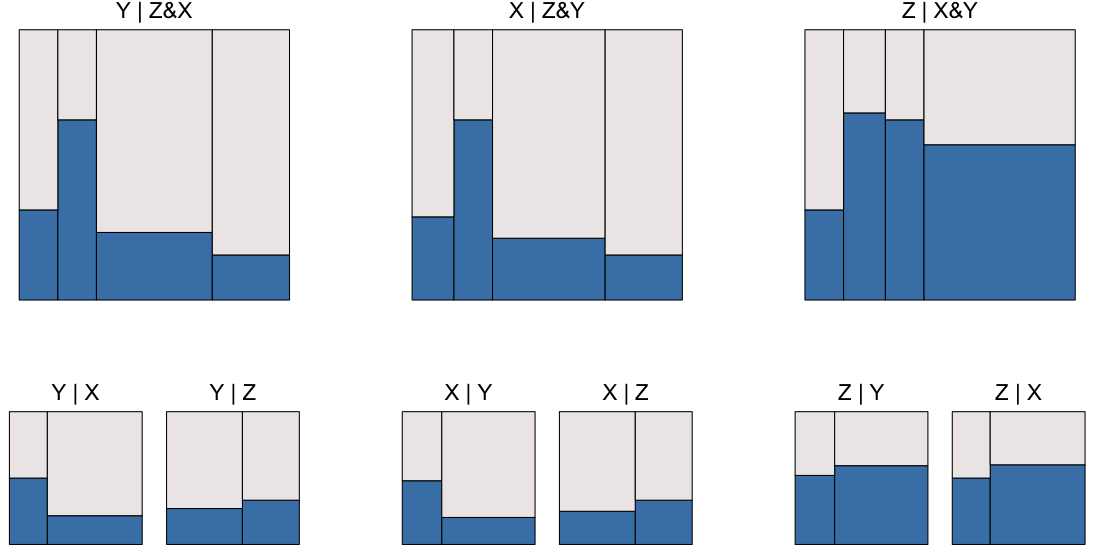
No flats; no marginal independence
There are no independencies present.
Case 4.2: No flats; one marginal independence
table <- create3WayBinaryTable(widths = c(1/4, 1/4, 1/4, 1/4),
                               heights = c(3/4, 1/2, 1/4, 1/4))

layout3and2way(table)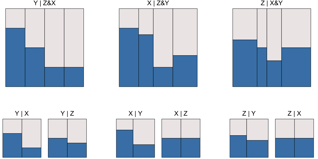
No flats; one marginal independence
Only independence is present is the marginal independence \(Z \bot\hspace{-.5em}\bot X\).
Note however that there is also a conditional indepenence but only for a single value of the conditioning variate, namely \(Y \bot\hspace{-.5em}\bot Z ~\vert~(X = x2)\), which can be seen in the first eikosogram of the top row.
Case 4.3: No flats; two marginal independences
table <- create3WayBinaryTable(widths = c(2/6, 1/6, 2/6, 1/6),
                               heights = c(2/3, 1/2, 5/6, 1/6))

layout3and2way(table)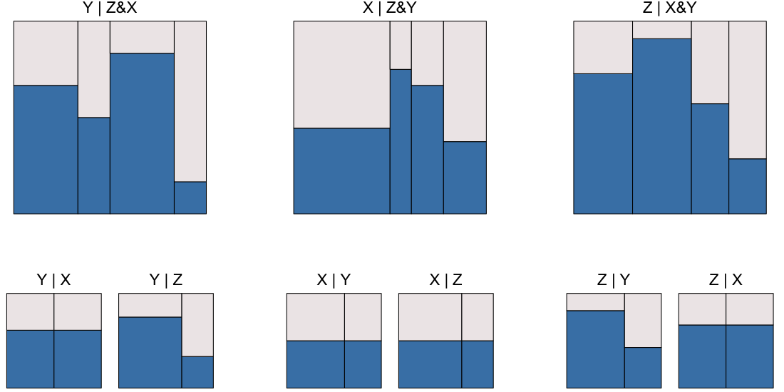
No flats; two marginal independences
Two marginal independences exist, \(X \bot\hspace{-.5em}\bot Y\), and \(X \bot\hspace{-.5em}\bot Z\).
Case 4.4: No flats; three marginal independences
table <- create3WayBinaryTable(widths = c(1/6, 2/6, 1/6, 2/6),
                               heights = c(1/6, 2/3, 5/6, 1/3))

layout3and2way(table)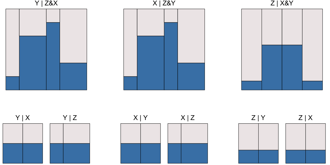
No flats; three marginal independences
All variates are pairwise independent but are not mutually independent. That is, \(X \bot\hspace{-.5em}\bot Y\), \(Y \bot\hspace{-.5em}\bot Z\), and \(X \bot\hspace{-.5em}\bot Z\) but \(\bot\hspace{-.5em}\bot\hspace{-0.85em} \times (X, Y, Z)\). No conditional independence exists.