The K distribution

R. Wayne Oldford

Definition

Suppose $X \sim \chi^2_m$ is a Chi-squared random variate on $m$ degrees of freedom. Then the distribution of $$Y = \sqrt{\frac{X}{m}}$$ is the Kay distribution on $m$ degrees of freedom, written as $$Y \sim K_m.$$ Its density is $$f(y) = \left\{\begin{array}{lcl} \frac{m^{\frac{m}{2}} y ^{m-1} e^{-\frac{1}{2} m y^2}} {2^{\frac{m}{2}-1} \Gamma(\frac{m}{2})} &~~~& \text{for} ~~ 0 \le y < \infty \\ &&\\ 0 && \text{otherwise}. \end{array} \right.$$

The $K_m$ density has some very attractive features over the $\chi^2_m$ density:

• $K_m$ has a much more symmetric density than had the $\chi^2_m$, for any $m$;
• like a $\chi^2_m$ density a $K_m$ density, as $m \rightarrow \infty$$K_m$ becomes more symmetric and nearly normally distributed but does both faster than a $\chi^2_m$;
• as $m \uparrow$, the $K_m$ density concentrates around the value $y=1$, rather than heading off to $\infty$ like the $\chi^2_m$;

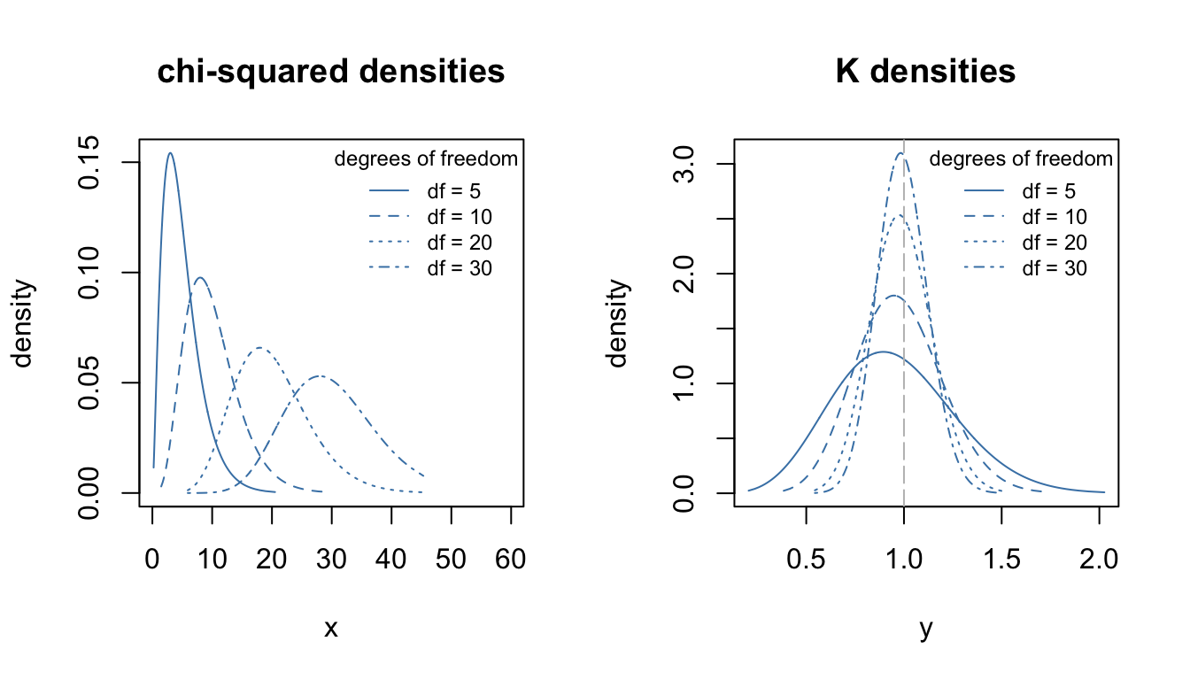
As m increases, Km has better properties

These values were calculated using the dkay(...) density function. For example, dkay(1.0, df=10) = 1.7546737.

Normal theory relations

Perhaps the most obvious relation between a normal random variate and a $K_m$ is that if $Z \sim N(0,1)$, then $|Z|\sim K_1$, the half-normal.

More important in applications is that distribution of the estimator of the sample standard deviation is proportional to a $K_m$. To be precise, if $Y_1, \ldots, Y_n$ are independent and identically distributed as $N(\mu, \sigma^2)$ random variates, with realizations $y_1, \ldots, y_n$ and the usual estimates $\widehat{\mu} = \sum y_i /n$ and $\widehat{\sigma} = \sqrt{\sum (y_i - \widehat{\mu})^2/(n-1)}$, then the corresponding estimators $\widetilde{\mu}$ and $\widetilde{\sigma}$ are distributed as $$\widetilde{\mu} \sim N(\mu, \frac{\sigma^2}{n}) ~~~~~\text{and} ~~~~~ \frac{\widetilde{\sigma}}{\sigma} \sim K_{n-1}.$$ The latter shows that $K_m$ is used for inference (e.g. tests and confidence intervals) about $\sigma$.

This is handy because the $K_m$ quantiles vary much less than do those of $\chi^2_m$. For example, condider the following table of the cumulative distribution.

df	p=0.05	p=0.5	p=0.95
1	0.0627068	0.6744898	1.959964
2	0.2264802	0.8325546	1.730818
3	0.3424648	0.8880642	1.613973
4	0.4215220	0.9160641	1.540108
5	0.4786390	0.9328944	1.487985
6	0.5220764	0.9441152	1.448654
7	0.5564364	0.9521263	1.417601
8	0.5844481	0.9581311	1.392269
9	0.6078297	0.9627987	1.371090
10	0.6277180	0.9665308	1.353035
15	0.6957463	0.9777136	1.290886
20	0.7365735	0.9832962	1.253205
25	0.7644974	0.9866425	1.227232
30	0.7851255	0.9888719	1.207932
35	0.8011601	0.9904636	1.192858
40	0.8140839	0.9916570	1.180662

Unlike the $\chi^2_m$ distribution, the quantiles in this table stabilize, allowing $1 \pm 0.20$ being not a bad rule of thumb for a $90\%$ probability of the ratio $\widetilde{\sigma}/\sigma$.

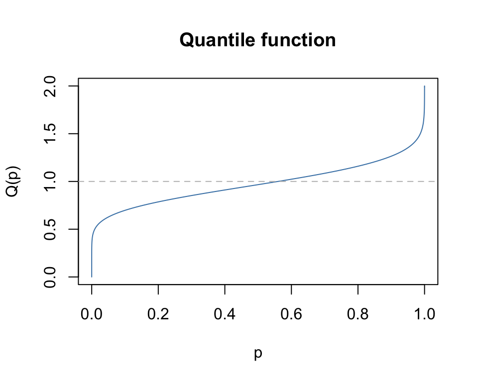
These values were calculated using the qkay(...) quantile function. For example, qkay(0.05, df=5) = 0.478639. These would be used to construct interval estimates for $\sigma$.

To get observed significance levels, the cumulative distribution function pkay(...) would be used. For example, SL = 1- pkay(1.4, df=10) = 1 - 0.9667287 = 0.0332713.

The Student t distribution

For the standard normal theory, the Student $t_m$ distribution can be defined as follows. If $Z \sim N(0,1)$ and $Y \sim K_m$ is distributed independently of $Z$, then the ratio $$T=\frac{Z}{Y} = \frac{N(0,1)}{K_m} = t_m$$ which is fairly easy to remember.

For the estimators from the above model $$\frac{\widetilde{\mu} - \mu} {\widetilde{\sigma} / \sqrt{n}} = \frac{ \frac{\widetilde{\mu}-\mu} {\sigma/\sqrt{n}} } {\frac{\widetilde{\sigma}} {\sigma} } = \frac{N(0,1)}{K_{n-1}} = t_{n-1}$$ is used to construct interval estimates and tests for the value of the parameter $\mu$.

The functions

As with every other distribution in R four functions are provided for the $K_m$ distribution. These are

• dkay(x, df=m, ...) which evalutes the density of $K_m$ at $x$,
• pkay(x, df=m, ...) which evalutes the distribution of $K_m$ at $x$,
• qkay(p, df=m, ...) which evalutes the quantile of $K_m$ at the proportion $p$,
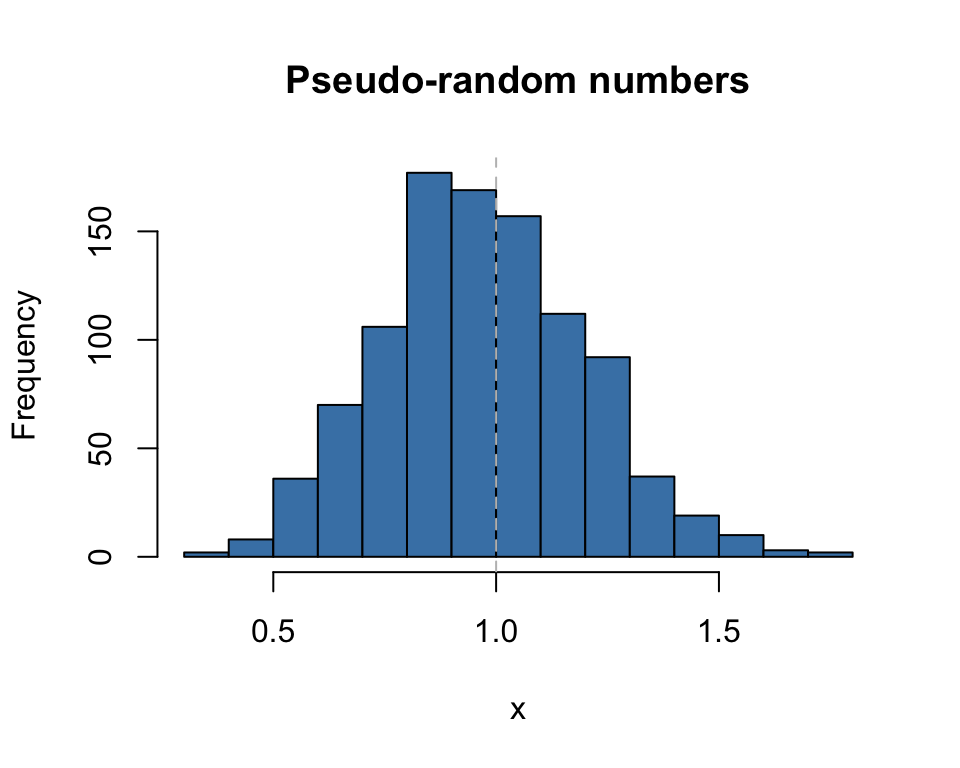
• rkay(n, df=m, ...) which generates $n$ pseudo-random realizations from $K_m$.

The parameters in the ellipsis include a non-centrality parameter. All functions rely on the corresponding $\chi^2_m$ functions in base R.

We briefly illustrate each below.

The density dkay(x, df, ...)

x <- seq(0,2,0.01)
plot(x, dkay(x, df=10), type="l", col="steelblue", 
     main="Density", xlab="x", ylab="f(x)")
abline(v=1.0, lty=2, col="grey")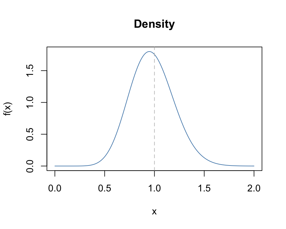

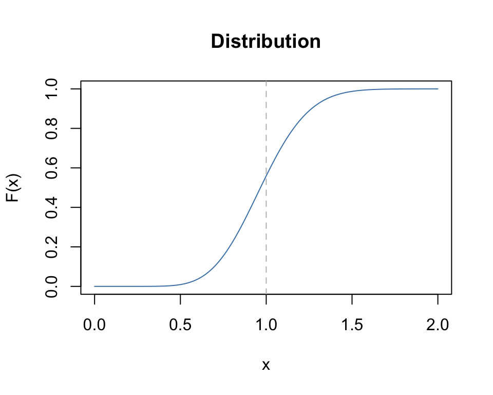
The cumulative distribution function pkay(x, df, ...)

x <- seq(0,2,0.01)
plot(x, pkay(x, df=10), type="l", col="steelblue", 
     main="Distribution", xlab="x", ylab="F(x)")
abline(v=1.0, lty=2, col="grey")

The quantile function qkay(p, df, ...)

x <- seq(0,2,0.01)
p <- pkay(x, df=10)
plot(p, qkay(p, df=10), type="l", col="steelblue", 
     main="Quantile function", xlab="p", ylab="Q(p)")
abline(h=1.0, lty=2, col="grey")

Pseudo-random realizations rkay(n, df, ...)

x <- rkay(1000, df=10)
hist(x, col="steelblue", 
     main="Pseudo-random numbers", xlab="x")
abline(v=1.0, lty=2, col="grey")